Linear Autoencoders and the Identity

This post assumes familiarity with linear algebra at the level of my post on low rank matrices.

Introduction

I recently read a wonderful paper by Netflix on linear autoencoders (LAEs), and how to avoid them overfitting towards the identity¹. The paper also discusses how LAEs perform low rank approximation of a matrix, and relate to previous matrix factorisation (MF) techniques.

Here’s I’ll dive into the main results of the paper, elaborating on some of the points, and augmenting them with pytorch code to make things more concrete. Overall I think this post could lead to a more fleshed out understanding of some really fundamental ideas.

The Setup

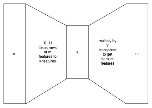
The basic idea is that we have a data matrix $X \in R^{r, m}$, where each row is an example with $m$ features. We want to find a lower rank $B=UV^T$ where $B \in R^{m,m}, U, V \in R^{m,k}$, and $k \lt\lt m$. So each row of $X$ has $m$ features that are compressed to $k$ features. $U$ encodes and $V^T$ decodes, since we want find $B$ to minimise

$$|| X - X \cdot B ||_F^2$$

If $k=m$ the obvious solution is the identity, $B = I_m$. Presumably a low rank approximation will also tend to the identity as much as possible. Graphically this can be seen as a linear autoencoder:

The paper looks at two key extensions to this:

1. Introduce dropout on the data matrix. In other words, for example $u$, dropout the feature $i$ with probability $p$, where

$$ Z_{u,i} = \delta_{u,i} \cdot X_{u,i} $$

and $\delta_{u,i}$ is a Bernoulli random variable. The idea here is that $B$ then needs to learn to recover $X_u$ without feature $i$.

2. Use what’s called “emphasis”. In other words, seek to minimise

$$ || A^{1/2} \odot (X - Z \cdot B) ||_F^2$$

Remember in this case $Z$ effects the dropout from point (1). $\odot$ is element wise multiplication. $A$ simply weights how much we care that each entry’s reconstruction deviates from the actual value. We let $A_{u,i}=a$ when there’s dropout ($\delta_{u,i}=0$), and $b \leq a$ otherwise. If $a=b$, we don’t mind if the feature is reconstructed from itself (tending to the identity) or other features. If $a > b$ then the loss will be higher when we fail to reconstruct a feature from other features.

In reality the author expresses the objective function above as the average of $n$ duplicates by vertically stacking the matrices to reflect gradient descent, but I don’t want to add complexity to the notation.

LAE in code

We can set up a linear autoencoder in Google Collab as follows:

import time
import torch
import torch.nn as nn
from torchvision import io, transforms, datasets
import matplotlib.pyplot as plt
%matplotlib inline

# set random seed for reproducibility
torch.manual_seed(42)
if torch.cuda.is_available():
    torch.cuda.manual_seed_all(42)

# set the device
device = torch.device('cuda:0' if torch.cuda.is_available() else 'cpu')

# define the LAE
class AutoEncoder(nn.Module):
    def __init__(self, input_dim, encoding_dim):
        super(AutoEncoder, self).__init__()
        self.encoder = nn.Linear(input_dim, encoding_dim)
        self.decoder = nn.Linear(encoding_dim, input_dim)

    def forward(self, x):
        x = self.encoder(x)
        x = self.decoder(x)
        return x

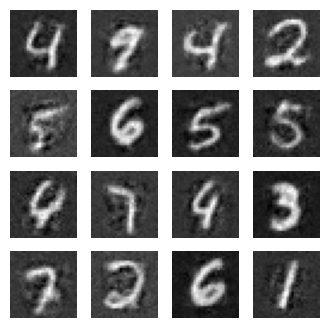
Next we’ll use the famous MNIST dataset of written digits that look like this:

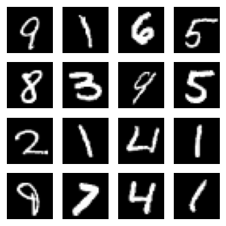
We download the data, convert it into tensors and normalise (which tends to improve convergence). We then set it up for training. Notice we’re taking a smaller sample of the data just to speed things up for demonstration. Each image has one channel of colour (grayscale), and dimensions $28*28=784$.

# Set a smaller number of training samples (e.g., 5000) to speed up training
# default set has around 60k images, test set has about 1k
smaller_num_samples_train = 5000
smaller_num_samples_test= 200
num_epochs = 100 # set consistent training epochs for all runs
batch_size = 64

datasets.MNIST(root="./MNIST_data", train=True, download=True)

# Create training and test data loaders
# Normalising the data can help with training convergence
transform = transforms.Compose([transforms.ToTensor(), transforms.Normalize((0.1307,), (0.3081,))])

# The DataLoader objects handle batching and shuffling of the data during training and testing.
trainset = datasets.MNIST(root="./MNIST_data", train=True, download=True, transform=transform)
trainset.data = trainset.data[:smaller_num_samples_train]
trainset.targets = trainset.targets[:smaller_num_samples_train]
trainloader = torch.utils.data.DataLoader(trainset, batch_size=batch_size, shuffle=True)

testset = datasets.MNIST(root="./MNIST_data", train=False, download=True, transform=transform)
trainset.data = testset.data[:smaller_num_samples_test]
trainset.targets = testset.targets[:smaller_num_samples_test]
testloader = torch.utils.data.DataLoader(testset, batch_size=batch_size, shuffle=True)

Before training, let’s instantiate our simple autoencoder, and see what results it produces with random weights. Notice we aren’t doing any compression for now, so $k=m$. Also pay close attention to code like .to(device), .cpu() or .cuda() to see where we do GPU computation to speed things up. We also need to set Google Collab’s runtime to explicitly use a GPU. .detach() is used when we want to ignore gradients for backprop.

# start with no compression
input_dimension = 1*28*28
input_dim = input_dimension
encoding_dim = input_dimension

autoencoder = AutoEncoder(input_dim, encoding_dim)
# send the weights to the gpu
autoencoder.to(device)

and plot:

# show reconstruction with random weights
num_images = 16
fig = plt.figure(figsize=(num_images // 4, 4))
for i, (images, labels) in enumerate(trainloader):
    for j in range(num_images):
        # ! add the image to the gpu as well
        input = images[j].view(28*28).cuda() # stack the input as one column of data
        image = autoencoder(input).view(28, 28) # view output as an image again
        fig.add_subplot(4, num_images // 4, j + 1)
        # send it back to the cpu to plot
        plt.imshow(image.cpu().detach().squeeze(), cmap='gray') # add detach to avoid gradient to numpy
        plt.axis('off')
    if i >= 1:
        break  # Exit the loop after displaying the first batch
plt.show()

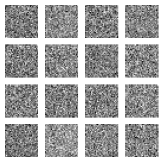
As expected, the autoencoder doesn’t yet know how to faithfully encode and then decode an image: we end up with noise. Let’s now train on minibatches.

# let's time the training as well
start_time = time.time()

# Define the loss function and optimizer
loss_function = nn.MSELoss()
optimizer = torch.optim.Adam(autoencoder.parameters(), lr=0.001)

for epoch in range(num_epochs):
    for i, (images, labels) in enumerate(trainloader):
        images = images.view(images.shape[0], -1).cuda() # convert to (example, stacked)

        optimizer.zero_grad()
        outputs = autoencoder(images)
        loss = loss_function(outputs, images)
        loss.backward()
        optimizer.step()

    if (epoch + 1) % 10 == 0:
        print(f'Epoch [{epoch + 1}/{num_epochs}], Loss: {loss.item():.4f}')


end_time = time.time()
execution_time = end_time - start_time
print('execution time: {}'.format(execution_time))

The run takes only 11 seconds on a T4 GPU, and our loss goes from 0.13 to 0.0067. If we print out $B$ we see the diagonal entries as being pretty close to 1, and off diagonal entries at least an order of magnitude smaller. So as speculated $B$ does seem to tend to the identity matrix.

The reconstructions look pretty similar to the original digits since we aren’t really doing any compression:

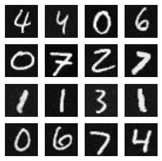
What happens if we set $k \lt\lt m$, for example $64 \lt\lt 784$? Impressively, we still get pretty good reconstructions, but as expected there is some compression loss:

Denoising Linear Autoencoder (DLAE)

Recall our objective function when we have an emphasis matrix $A$ and a dropout matrix $Z$ that occasionally hides a feature in the training set:

$$ || A^{1/2} \odot (X - Z \cdot B) ||_F^2$$

All entries in $A$ are equal, they have no effect on the optimal $B$. Then only dropout is at play, and it’s called a denoising autoencoder. Specifically, since it’s linear, we have a denoising linear autoencoder (DLAE). It’s denoising because we’re introducing noise through dropout, then trying to denoise it. Dropout is actually a very specific type of noise: omission that is independent across examples and features. In theory we could add other types of correlated noise. That’s why I wish it were called a “dropout linear autoencoder” instead of “denoising”. But at least the acronym sort of works out either way!

It turns out² that denoising is the same as $L_2$ regularisation on the matrix $B$, with a very specific interpretation of the regularisation weights. Specifically,

$$ \hat{B}^{(DLAE)} = \mathop{\arg \min}\limits_{B} ||X - X \cdot B||_F^2 + ||\Lambda^{1/2} \cdot B||_F^2 $$ where $\Lambda=\frac{p}{q} \cdot diagmatrix (X^T \cdot X)$. Here I use the function $diagmatrix$ that takes the diagonal of the argument, and turns that into a diagonal square matrix.

More on $\Lambda$

So what does the diagonal matrix of regularisation weights do? First let’s parse the shapes to make sure we are thinking about what’s going on. Remember $X$ has shape $(r, m)$ (in pytorch syntax), so $X^T \cdot X$ gives us a matrix of second moments of shape $(m, m)$. Second moments is just fancy terminology for something like a covariance matrix, but where we haven’t subtracted any means or averaged. The covariance matrix would normally be $\frac{1}{r-1} (X - \mu)^T \cdot (X - \mu))$ ³.

Notice that we’re averaging each feature across training examples, not each training example across features. Now recall that by left multiplying $B$ with a diagonal matrix, we’re just scaling each row by the corresponding diagonal element. So the higher the variance of a feature, the smaller we want that row in $B$. Put differently, higher variance features are regularised more.

Minimising things of the form $||X-X \cdot B||_F^2 + ||constants \cdot B||_F^2$ is also known as ridge regression, or $L_2$ regularisation, and has a closed form solution. If $B$ is fullrank in particular, the solution to the ridge regression problem is as follows. Basically the trick (not shown here) is to take the loss with regularisation, set the gradient to zero, and get our starting point below.

The full rank case can be seen as a limiting case of $B$ with a lower rank, and so is still useful for analysis:

$$ \begin{align*} \hat{B}_{full}^{(DLAE)} &= (X^TX + \Lambda)^{-1} X^TX \\ &= \cdots \\ &= I - (X^TX + \Lambda)^{-1}\Lambda \end{align*} $$

What does this tell us? With no regularisation, the solution wants to be the identity. Otherwise, the second term allows for non-diagonal entries to be non-zero, and possibly reduces diagonal entries.

Does DLAE take us further from the identity?

Without dropout, in our earlier example with compression ($k=64$) we can see how much the diagonal of $B$ deviated from the identity matrix:

def diff_from_I(model):
  with torch.no_grad():
    # B = UV^T
    B = model.encoder.weight @ model.decoder.weight
    # print(torch.diag(B))
    # print(B[0])

    diff_from_I = torch.norm(torch.diag(B) - torch.eye(B.shape[0]).cuda(), p='fro') / B.shape[0]
    print('diff from identity (norm): {}'.format(diff_from_I))

print(diff_from_I(autoencoder))

The mean squared error (MSE) from the identity is 0.66. Let’s now add dropout to our autoencoder and see if we get further from the identity. Notice that we can add the dropout layer at various points. In this case we’re adding it to the input layer: for a given input, any of the $m$ features can be dropped out, which is what we want.

class AutoencoderWithDropout(nn.Module):
    def __init__(self, input_dim, encoding_dim, dropout_rate=0.2):
        super(AutoencoderWithDropout, self).__init__()
        self.dropout = nn.Dropout(dropout_rate)
        self.encoder = nn.Linear(input_dim, encoding_dim)
        self.decoder = nn.Linear(encoding_dim, input_dim)

    def forward(self, x):
        x = self.dropout(x)
        x = self.encoder(x)
        x = self.decoder(x)
        return x

Important note: when training with dropout, neurons are ommitted randomly during a training run with probability $p$. However during inference, all neurons are active, so activations add up to bigger numbers. To scale this so that the expected value of the output remains the same, we need to multiply weights⁴ by $1-p$. The default pytorch dropout layer makes this easy: remember to run model.train() before training, and model.eval() before inference. Under the hood, this sets the model.training boolean. This can be a source of silent bugs!

With dropout, the MSE from the identity goes down to 0.51 verus 0.66 before. In practice we should be doing more comprehensive tests on a number of training runs and models, but this does indicate that indeed dropout pulls $B$ away from the identity.

The author also goes on to claim that DLAE is better than “weight decay”, because the former regularises $||B = U \cdot V^T||$ while the latter regularises $||U||$ and $||V||$ separately. Thus DLAE is invariant to various compressions of the same rank, and leads to better accuracy. In addition, as we saw with $\Lambda$, regularisation varies by feature, as opposed to some global constant $\lambda$.

Next let’s look at whether emphasis pulls us even further from the identity.

Emphasis (EDLAE)

By introducing the weightings $A$, we turn the system into an emphasised (denoising) linear autoencoder (ELDAE) if $a \gt b$. We would then be emphasising reconstructing a given feature from other features, since the loss would be higher for cases where the feature itself was dropped out.

The author goes on to show this algebraically, decoupling the $L_2$ regularisation in general, form the emphasis matrix pulling $B$ away from the identity.

EDLAE in code

How can we introduce an emphasis matrix intro our loss function? First, we need to get the dropout mask from our dropout layer. This isn’t natively provided, so we program a custom dropout layer. Notice we take into account whether we’re in training or inference mode:

class CustomDropout(nn.Module):
    def __init__(self, p=0.5):
        super(CustomDropout, self).__init__()
        self.p = p

    def forward(self, x):
        keep_prob = 1 - self.p
        random_tensor = torch.rand(x.size()).cuda()
        dropout_mask = random_tensor.lt(keep_prob)
        dropout_output = x.mul_(dropout_mask.float())
        if self.training is False:
          dropout_output = dropout_output.div_(keep_prob)
        return dropout_output, dropout_mask

Now we can use this in our model:

class AutoencoderWithDropout(nn.Module):
    def __init__(self, input_dim, encoding_dim, dropout_rate=0.2):
        super(AutoencoderWithDropout, self).__init__()
        self.dropout = CustomDropout(dropout_rate)
        self.encoder = nn.Linear(input_dim, encoding_dim)
        self.decoder = nn.Linear(encoding_dim, input_dim)
        self.dropout_mask = None

        self.emphasis_a = 2 # when feature is predicted without itself
        self.emphasis_b = 1

    def forward(self, x):
        x, dropout_mask = self.dropout(x)
        self.dropout_mask = dropout_mask
        x = self.encoder(x)
        x = self.decoder(x)
        return x

Next we need to use this dropout mask to weight our losses by either $b$ or $a \geq b$ for our “emphasis” mechanism. Dimensions can get tricky here. If feature $i$ out of $m$ features is dropped, we want to apply $a$ to that loss, else $b$. We implement our own loss function within the model this time. In case you spot it, the way I’m doing the calculation here uses $(a-b)$ and cancellation instead of using a complement of the dropout mask.

class AutoencoderWithDropout(nn.Module):
    ...

    def custom_mse_loss(self, true):
            pred = self(input)  # Get the model's predictions
            loss = (pred - true).pow(2) # squared differences
            a_loss = torch.mul(loss, self.dropout_mask * (self.emphasis_a - self.emphasis_b) # weight feature m deviation, elementwise
            b_loss = self.emphasis_b * loss
            loss = a_loss + b_loss
            loss = loss.mean()
            
            return loss 

Training once more, we deviate from the identity by a mean squared error of 0.12, as opposed to 0.51 for DLAE and 0.66 for LAE. Indeed we have moved away from the identity!

Conclusion

In this post we’ve explored the idea of compressing MNIST images with a linear autoencoder. We started with no compression, which worked well but had lots of parameters and tended to the identity.

After introducing compression, we added dropout and saw that this was equivalent to $L_2$ regularisation, which did pull us away somewhat from the identity. Finally we introduced arbitrary emphasis into our loss, and were able to learn the reconstruction of a certain feature relying on other features to an even greater extent.

Most of all, we implemented this in pytorch and saw illustrative results! Now that we have a feel for linear autoencoders, it might be fun to explore more sophisticated forms of compression. Even more interesting to me is exploring how representations and embeddings work in general - there’s a lot we still don’t understand in the field!

Footnotes