Low Rank Matrices, an Introduction

Introduction

I thought it would be fun to go over some matrix basics since they’re used everywhere. In particular, embeddings in machine learning are just lists of numbers. I’ve been investigating those of late, and it’s useful to be fluent with matrices when playing around with them.

I’ll start with very simple questions then move on to some slightly more advanced concepts. In this post in particular, I’d love to discuss the extremely useful notion of low rank matrices, and how we can decompose a matrix into its “ingredients”. We’ll find out what that means shortly and why it’s so cool.

What is a matrix?

The basics

A number on its own is called a scalar, or a 0-dimensional tensor, e.g. $7$.

If you have an ordered array of numbers, we call this a vector or a 1-dimensional tensor, e.g. $v = [7, 9, 3]$, where $v_0$ would index the first element $7$, $v_1$ would be $9$ and so on. In fact, vectors could even be abstract things that we just call $v$ or $w$ for example, that are members of a vector space. For now let’s assume we’re just dealing with numbers, which is usually the case in applied settings.

A 2-dimensional tensor, or 2-d array of numbers is called a matrix, e.g.

$$ M = \begin{bmatrix} 7 & 9 & 3 \\ 1 & 2 & 7 \\ 5 & 6 & -1 \\ 0 & -4 & 0 \end{bmatrix} $$

In this case the matrix has 4 rows and 3 columns, so we say its shape is (4, 3). Sometimes we write this as $M \in \mathbb{F}^{4,3}$ where $\mathbb{F}$ is a “field” like the real or complex numbers. $M_{i,j}$ would index the $i$‘th row and $j$‘th column. So $M_{0,1} = 9$ and so on. A word of caution: often vectors are 0-indexed whereas matrices are 1-indexed (the starting index), so more commonly we would actually have $M_{1,1} = 9$ above. Use context to figure things out, otherwise assume 1-indexing with matrices.

n-dimensional tensors would have $n$ indices, so if a 2-d array represents pixels of an image for example, a 3-d tensor could be a movie of images over time. We won’t get into tensors any further than that for now.

What does a matrix signify?

A matrix can be interpreted in many ways. Let’s explore some of the more common ones.

A bunch of data

Let’s say I ate 5 apples, 2 oranges, and 1 pear in a given week. Let’s represent this as a row vector of shape (1, n), as opposed to a column vector of shape (n, 1)). Unless otherwise specified, a vector is usually assumed to be a column vector. Here our row vector is: $[5, 2, 1]$. If I recorded my consumption over a number of weeks, I could organise these into a “data matrix” where each row is an “observation” (week). I was a bit less healthy that final week:

$$ \begin{bmatrix} 5 & 2 & 1 \\ 7 & 1 & 3 \\ 1 & 0 & 1 \end{bmatrix} $$

The key point here is that each row is the same thing: a week of my consumption. Likewise each column represents how many apples, oranges and pears I ate. It would not make sense to combine different meanings for different rows and columns into a matrix e.g. where some rows are a week, other rows a month, other rows a blood test; or where some entries in the first column represent my apple consumption, and others represent the temperature on a given day.

Simultaneous equations

Take your bunch of data, and assume you can use it to linearly estimate some “target”. For example, if we take our previous matrix of my fruit consumption across a few weeks, imagine each week I also recorded my cholesterol level. If my cholesterol happens to be a linear function of my fruit consumption, we could represent this as simultaneous equations:

$$ \begin{align*} 5x_1 + 2x_2 + 1x_3 &= 12 \\ 7x_1 + 1x_2 + 3x_3 &= 8 \\ 1x_1 + 0x_2 + 1x_3 &= 4 \end{align*} $$

This can be written more compactly in matrix form as $Ax = b$, representing the following matrix equation:

$$ \begin{align*} \begin{bmatrix} 5 & 2 & 1 \\ 7 & 1 & 3 \\ 1 & 0 & 1 \end{bmatrix} \begin{bmatrix} x_1 \\ x_2 \\ x_3 \end{bmatrix} &= \begin{bmatrix} 12 \\ 18 \\ 4 \end{bmatrix} \end{align*} $$

We want to find the coefficients in the vector $x$ that take us from fruit numbers to cholesterol. Units are important here: if we’re measuring cholesterol in grams/liter, and fruit in grams, then the coefficients technically have units in 1/liter for things to work out.

We can solve these simultaneous equations as per usual, where subtracting one equation by another represents doing so across rows of the matrix. Likewise multiplying an equation by a scalar means multiplying a row of $A$ and $b$ at the same time. Rows can also be swapped without changing the solution, since that’s the same as rearranging the equations.

Assuming there is a solution, this could be done with the following Python code. For such a small problem, one would probably use a library like numpy, but I’ll use pytorch here so we familiarise ourselves with its tensors which will be useful for machine learning. I like to use Google Collab to play around with such code, since it doesn’t require setting up an environment.

import torch

A = torch.tensor([
    [5,2,1],
    [7,1,3],
    [1,0,1]
], dtype=torch.float32)
b = torch.tensor([
    12, 18, 4
], dtype=torch.float32)

print(A.shape)
print(b.shape)
b = b.unsqueeze(1)
print(b.shape)
>>> torch.Size([3, 3])
>>> torch.Size([3])
>>> torch.Size([3, 1])

I honestly believe that a huge part of linear algebra (and therefore data science, machine learning etc.) is just about understanding the dimensions of tensors you’re manipulating. That’s partly because the notation is so overloaded; $Ax = b$ can feel like a regular equation, but it’s high dimensional¹. For example you can’t always “divide” by $A$, matrix multiplication isn’t always commutative, and dimensions have to align for it to make sense as we’ll see in more detail.

We set the data type of our tensors to float32 (a “long”) or we’ll get errors later down the line. If we don’t, they default to float64 (a “double”).

Above we see that $A$ has shape (3,3). Notice I’ve turned $b$ into a column vector (or matrix) of shape (3,1), instead of just an array of size 3. Why do this? It turns out this can be useful with broadcasting, matrix multiplication, and in terms of what type of input some pytorch functions expect, so I wanted to give a flavour of it here. That said we won’t worry about it too much for now.

Now that we have our data in tensors, we can seek to solve the system. Remember we want to find the coefficients in $x$.

x = torch.linalg.solve(A, b)

print(x)
print(x.shape)
print(torch.allclose(A @ x, b))
>>> tensor([[1.0000],
        [2.0000],
        [3.0000]])
>>> torch.Size([3, 1])
>>> True

The shape is as expected, and the last function allclose just checks that indeed the system is solved with these numbers. You should also verify this manually looking at the simultaneous equations. In summary, our solution is:

$$ \begin{align*} \begin{bmatrix} x_1 \\ x_2 \\ x_3 \end{bmatrix} &= \begin{bmatrix} 1 \\ 2 \\ 3 \end{bmatrix} \end{align*} $$

Graphs

I just wanted to mention it briefly since it’s a cool interpretation. If you imagined a graph with vertices labelled $0, 1, 2, \cdots, n$, then you could represent the graph as a matrix $G$ where entry $G_{i,j}$ is the weight on the edge from $i$ to $j$, and 0 might represent the absence of an edge. In the general case the edges are thus directed. If the matrix is symmetric (about its diagonal i.e. $G_{i,j} = G_{j,i}$), it could be interpreted as an undirected graph.

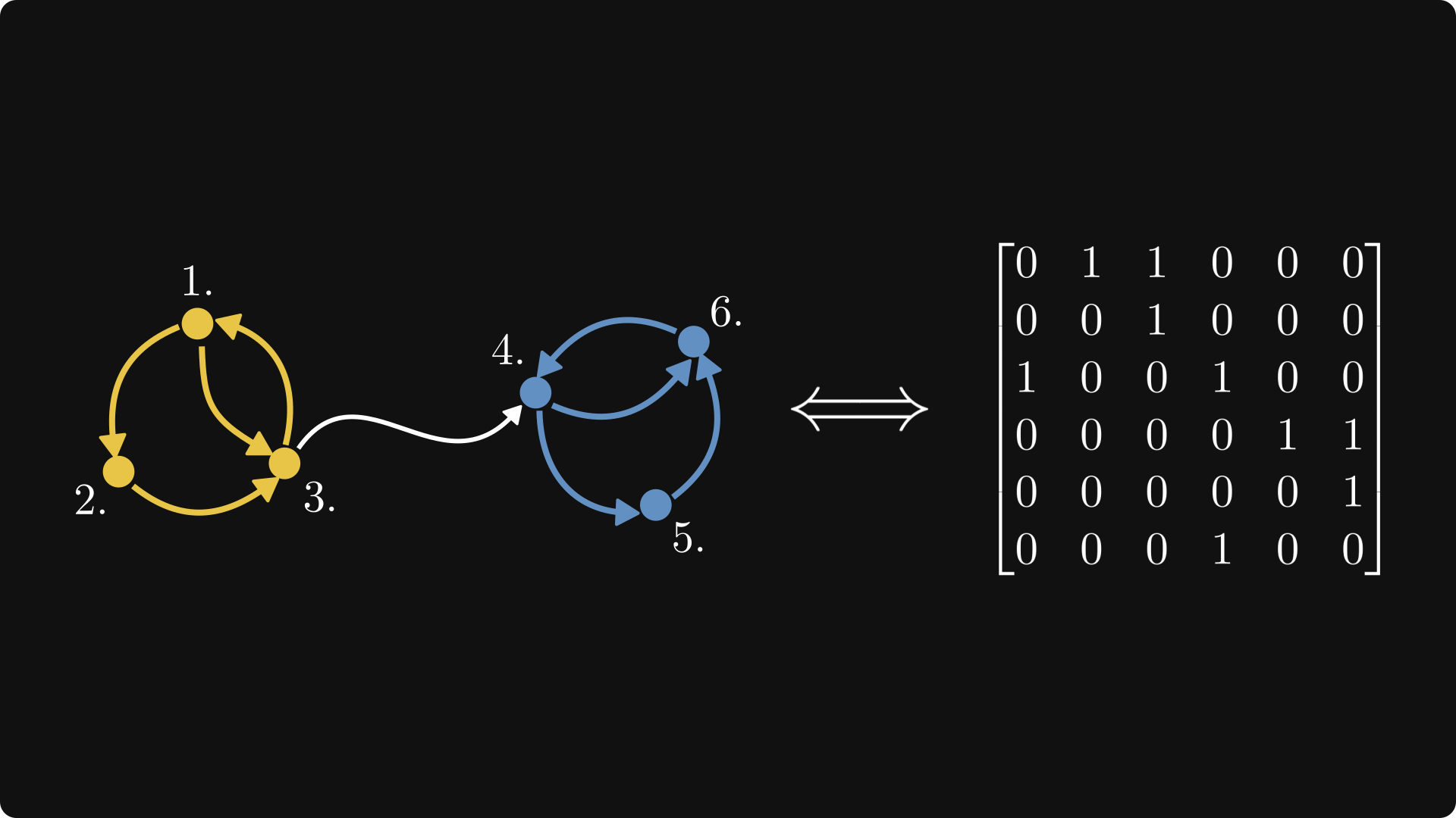
Example of a directed graph with equal edge weights of 1, and its matrix

Visualising some matrix multiplication

Matrix notation is powerful, but with great power comes great responsibility. It is exceedingly easy to read through some matrix equations without really thinking about what’s going on. To that end, I highly recommend always keeping track of the shapes of matrices, and visualising roughly what’s going on in terms of rows and columns. To that end, let’s visualise a few common operations.

Suppose we have a matrix $M$ of a linear transformation of shape (r,m). What happens when we left multiply a vector by it? I’ll sometimes use the @ symbol to denote matrix multiplication, since that’s common in pytorch. Carrying this out reveals that we are simply taking a linear combination of the columns with the vector providing the coefficients:

Likewise, if we multiply a row vector by a matrix, that vector gives us the coefficients for a linear combination of the matrix rows:

Another common operation involves diagonal matrices, often denoted by $\Lambda$. As we can see below, left multiplying by a diagonal matrix is like left multiplying by a row vector, except that instead of adding row multiples to end up with a row vector, we stack them into a new matrix!

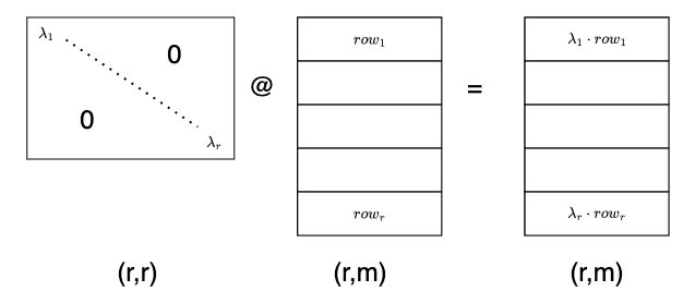
A right multiplication by a diagonal matrix does the same with the columns of the other matrix. Notice that the shape of this diagonal matrix is (m,m), which differs from the previous one with shape (r,r)!

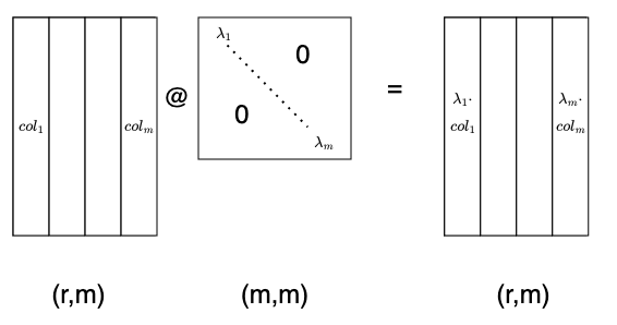
Now for contrast, compare this to the raw mathematical notation, where we reuse the input symbols $x$ and $y$ and so on even though they mean different things in each equation:

$$ \begin{align*} M \cdot x &= y \\ x_T \cdot M &= y \\ \Lambda \cdot M &= y \\ M \cdot \Lambda &= y \end{align*} $$

Again, it’s very, very easy to read those equations, believe all is dandy, and move on with life. But remember, a lot is going on here, even when it comes to basics like dimensions, let alone geometric and semantic interpretations!

Abstract linear transformations

Matrices can also be seen as transformations of vectors from one space to another. Loosely speaking, our example of simultaneous equations took a vector of linear coefficients $x$, and turned it into cholestorol measurements $b$ by applying our fruit matrix $A$. If I gave you a separate set of coefficients, you could likewise use $A$ to get new cholesterol predictions based on this new linear model. Interestingly in that case we’re not estimating coefficients; we’re estimating actual cholesterol measurements in given weeks from fruit consumption in those weaks, based on what you’re telling me the coefficients are. The matrix $A$ is thus a linear transformation from fruit consumption space to cholesterol space.

Let’s talk about linear transformations in a more abstract way now. I’m going to focus on the intuition, so please don’t sue me for minor imprecision.

Vector spaces

A vector space over a field $F$ is a set where addition between elements is defined, as well as scalar multiplication over the field. In other words, if $v, w \in V$, then you can take $v+w$ to get a new vector in $V$. You can also multiply $v$ by some $\alpha \in F$ (such as a complex number) to get $\alpha \cdot v \in V$. Addition is associative and commutative, and we have distributivity. This jibes with our intuition when working with vectors of numbers.

Furthermore, adding (the additive identity) $0$ to anything does nothing to it. Multiplying anything by (the multiplicative identity) $1$ also does nothing to it. Careful now, $0$ is a vector in $V$, while $1$ is the scalar in $F$. I wouldn’t be surprised if some pros occasionally missed this in parsing an equation! Finally every element $v \in V$ has an additive inverse $-v$ where $v + (-v) = 0 \in V$.

Linear transformations

The set of linear transformations from a vector space $V$ to another $W$ is denoted $\mathscr{L}(V,W)$. For example, $V$ could be $R^n$ and $W$ could be $R^m$, and the matrix for the transformation would have shape (m, n): it takes a vector in $R^n$ and turns it into a vector in $R^m$ which is a linear combination of the matrix’s columns as we saw earlier.

What is a linear transformation in the abstract sense? It’s one that satisfies:

1. linearity: $T(u+v) = T(u) + T(v)$
2. homogeneity: $T(\alpha v) = \alpha T(v)$, where $\alpha \in F$.

I like to summarise this as $T(\alpha v + \beta w) = \alpha T(v) + \beta T(w) $.

Let’s say every vector in $V$ can be represented as a unique combination of vectors $v_1, …, v_n$. Then we call $v_1, …, v_n$ a basis of $V$. The vectors in a basis can’t be represented in terms of each other (are linearly independent), which guarantees the unique representation. All bases also have the same dimension (number of vectors). In $R^n$, $e_1, …, e_n$ is an example of a (orthonormal) basis, where $e_i$ is a column vector of all zeros expect the i’th position (using 1-indexing).

To make this concrete, consider a 2-d vector $\begin{bmatrix}-2 \\ 1\end{bmatrix}$. This can be represented as $-2 * \begin{bmatrix}1 \\ 0\end{bmatrix} + 1*\begin{bmatrix}0 \\ 1\end{bmatrix}$. There’s no other way to represent the vector in terms of this basis of “ingredients”.

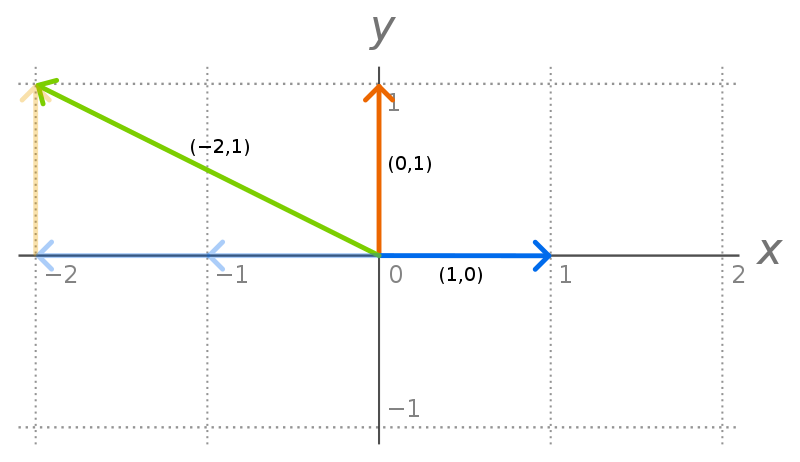
The standard basis² in $R^2$

So if I had a vector in $R^3$ (such as my fruit consumption), call it $\begin{bmatrix}3 \\ 4 \\ 2 \end{bmatrix}$, and wanted to transform it linearly into a vector in $R^2$ of cholesterol and blood sugar levels, I would multiply this by a matrix of shape (2, 3). Can this be made general for all vector spaces? Why yes!

Imagine $\begin{bmatrix}3 \\ 4 \\ 2 \end{bmatrix}$ now represents coordinates of a basis $v1_, v2, v3$ in some arbitrary 3-d vector space V, and we want to linearly transform it onto another vector space $W$ with its own basis vectors $w_1, w_2$. What does a matrix $M$ do to each basis vector? Well $v_1$ can be represented as $\begin{bmatrix}1 \\ 0 \\ 0 \end{bmatrix}$ in these coordinates. This selects out the first column of $M$ as we’ve seen.

By definition $M \cdot v_1 = T(v_1)$. Thus we see that the matrix of the transformation with respect to these chosen bases has as columns precisely the transformations of $V$’s basis vectors. That’s what the matrix represents! In fact every matrix represents a linear transformation, and every linear transformation has a matrix. They are one in the same by virtue of how linear transformations and matrices are defined.

Just a tad more terminology

Vectors that get mapped by $T$ to $0 \in W$ are part of what we call the nullspace or kernel of $T$, written $null(T)$.

The outputs of $T$ in $W$ constitute the range of $T$, written $range(T)$.

We’ll use this when discussing least squares.

Least squares

Now that we have a bit of an understanding of what matrices represent, I thought it would be fun to revisit the case of simultaneous equations, but where an exact solution is not possible. In other words, where we can only find an approximate “least squares” solution.

What does it mean if $Ax=b$ has no solution? It means that there’s no $x$ input that will get us the output $b$ through the linear transformation $A$. In other words, it means $b \notin range(A)$.

$Ax$ is basically all possible combinations of the columns of $A$. If $A$ has shape (r, m), then each column has $r$ numbers. Thus the combination of $A$’s columns in some subspace (possibly the whole space) in $R^r$. Thus we can visualise $range(A)$ as some subspace or plane, using $R^3$ as an example. $b \notin range(A)$ means it sits outside this subspace:

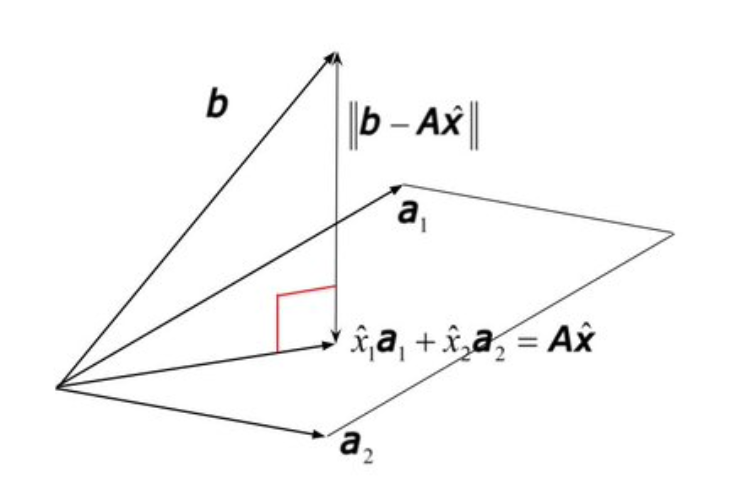
Projection of $b$ onto $range(A)$. We’re in the target space here!

Thus even if we can’t find $x$ to solve $Ax=b$ exactly, we can do the next best thing: find the closest point in $range(A)$ to $b$. This amounts to minimising the squares distance with high-dimensional Pythagoras.

$$ \begin{align*} || Ax - b ||^2 &= (Ax - b)^T \cdot (Ax - b) \\ &= x^T A^T A x - 2 b^T Ax + b^T b \end{align*} $$

We can set the gradient to zero:

$$ \nabla_x || Ax-b||^2 = 2 A^T Ax - 2A^T b = 0 $$

which gives us the “normal equations” $A^T A x = A^T b$. In other words, our “least squares” estimate of $x$ is $x_ls = (A^T A)^{-1} (A^T) b$. Notice we’ve assumed $A$ is “full rank” here. The rank is the number of linearly independent rows or columns (turns out they’re the same). Full rank means the rank is the maximum it could be, i.e. min(dimensions).

Thus the closest we can get to $b$ in the range of $A$ is $A \cdot x_{ls} = A (A^T A)^{-1} A^T b$, where the part before $b$ is the projection matrix, that projects $b$ to its closest point in the range of $A$, also known as $Proj_{A}(b)$.

Example with some code

Let’s recall our simultaneous equation example. This time, I’ll choose a $b$ that’s not in the range of $A$, and solve for least squares. I’ve chosen an $A$ of shape (3,2). That way its maximum rank is 2, while its target space is 3-d, so I know I can find something not in the range.

import torch

A = torch.tensor([
    [1,2],
    [1,3],
    [2,6]
], dtype=torch.float32)
b = torch.tensor([
    0, 1
], dtype=torch.float32)

What happens if we try to solve this system as before?

x = torch.linalg.solve(A, b)

---------------------------------------------------------------------------

RuntimeError                              Traceback (most recent call last)

<ipython-input-3-9ea5e4abce97> in <cell line: 1>()
----> 1 x = torch.linalg.solve(A, b)

RuntimeError: linalg.solve: A must be batches of square matrices, but they are 3 by 2 matrices

Ok it’s expecting a square matrix, so I’m guessing its expecting a full rank square matrix so it knows it can solve it. What happens if I give it a third linearly dependent column instead (say by adding the first two)?

A = torch.tensor([
    [1,2, 3],
    [1,3, 4],
    [1,0, 1]
], dtype=torch.float32)

b = torch.tensor([
    0, 7, 1
], dtype=torch.float32)

x = torch.linalg.solve(A, b)

print(x)
print(torch.allclose(A @ x, b))
print(torch.norm(A@x - b))

>>> tensor([[-2.4159e+08],
        [-2.4159e+08],
        [ 2.4159e+08]])
>>> False
>>> tensor(66.4906)

We see that the solution does not in fact solve for the equations! The numbers also look odd. Finally the solution is 66 units of distance away from $b$. Let’s find out what happens if we do least squares instead (with a non full rank $A$)!

x_ls = torch.linalg.lstsq(A, b).solution

# print statements...
>>> tensor([[ 24.8095],
        [-16.7619],
        [  8.0476]])
>>> False
>>> tensor(19.2428)

The numbers look more reasonably. We still don’t land on $b$, but the norm distance is a lot lower. Do we dare visualise $b$ and the range of $A$?

import numpy as np
import matplotlib.pyplot as plt
from mpl_toolkits.mplot3d import Axes3D

b_numpy = b.numpy()
A_numpy = A.numpy()

fig = plt.figure()
ax = fig.add_subplot(111, projection='3d')


# Plot range(A)
ax.plot_surface(np.arange(A_numpy.shape[0]), np.arange(A_numpy.shape[1]), A_numpy, cmap='viridis', edgecolor='none')

# Plot the vector b starting from origin (0, 0, 0)
ax.quiver(0, 0, 0, *b_numpy, color='r', arrow_length_ratio=0.2)

ax.set_xlim([-1, 1])
ax.set_ylim([-1, 10])
ax.set_zlim([-1, 1])

ax.set_xlabel('X')
ax.set_ylabel('Y')
ax.set_zlabel('Z')


plt.show()

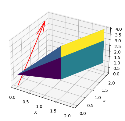
It’s not pretty, but we get the idea that $b$ (the red arrow) doens’t lie in the weird polygon that is $range(A)$.

Low rank matrices

We’re now linear algebra pros (or at least getting there), and can finally discuss low rank decompositions of a matrix.

Why do these matter? They come up in compression techniques, including linear autoencoders which I hope to discuss in a future post. Essentially, if we have a data matrix $X$ of shape (r,m) representing examples each with $m$ features, we may wish to embed these features into a smaller space of dimension $k « m$ so as to have more data per unit volume, and thus learn patterns better.

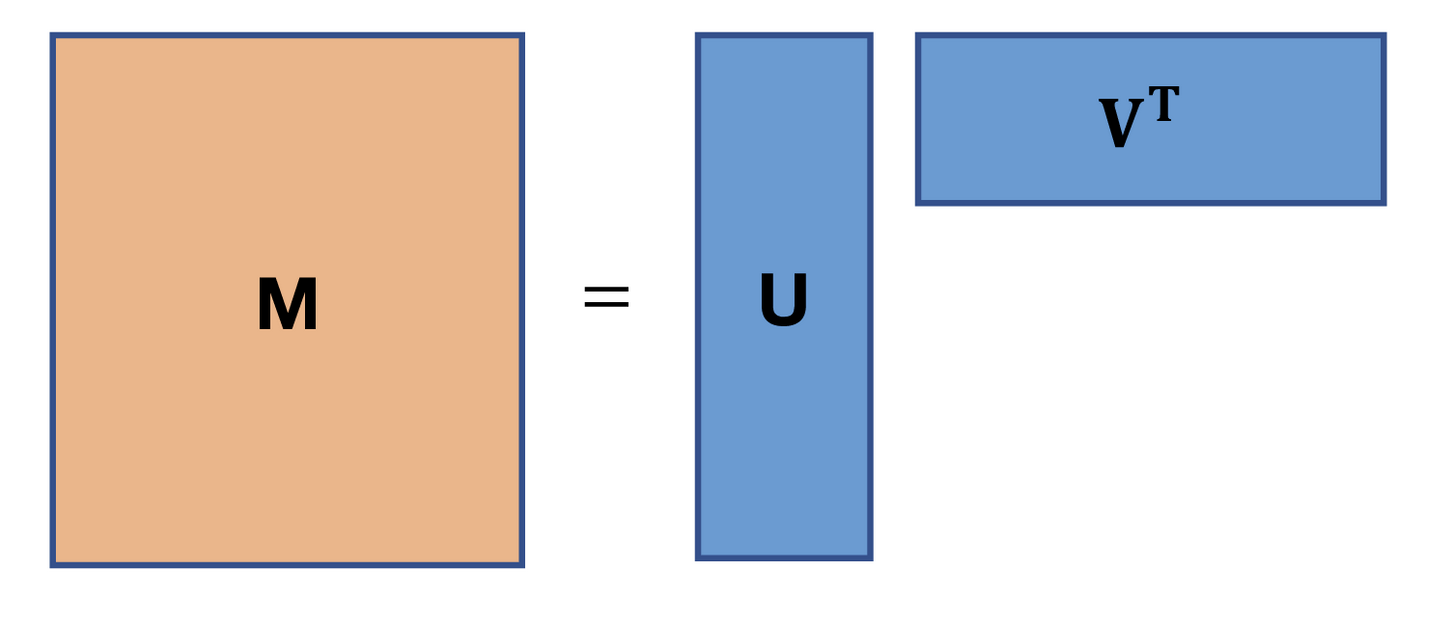
But let’s not get ahead of ourselves. For now, let’s just look at how a matrix can be made up of smaller, lower rank ingredients³. Imagine our $A$ has rank 1, that is all its rows are multiples of a single row, and likewise for its columns. We can then represent it as an outer product of $u$ with shape (r,1) and $v$ with shape (1, m):

$$ A = u \cdot v^T = \begin{bmatrix} | \\ u \\ | \end{bmatrix} \cdot \begin{bmatrix}—v^T—\end{bmatrix} = \begin{bmatrix}— u_1 v^T—\\—u_2 v^T—\\ \vdots \\ —u_r v^T— \end{bmatrix} = \begin{bmatrix}| & | & & | \\ v_1 u & v_2 u & \dots & v_m u \\ | & | & & | \end{bmatrix} $$

Likewise, if $A$ has rank 2, we can stack this idea and write $A$ as follows:

$$ A = \begin{bmatrix}| & | \\ u & w \\ | & |\end{bmatrix} \cdot \begin{bmatrix}—v^T— \\ —z^T—\end{bmatrix} $$

Thus we retrieve the cover image of this blogpost, where $A$ of rank $k < min(r,m)$ can be rewritten as a product of two rank $k$ matrices:

Conclusion

We’ve gone over matrix notation and various interpretations of matrices, including more abstract theory. We’ve also worked hard to engage with the notation, thinking about matrix shapes and visualising what’s going on. Finally, we applied some of these ideas in pytorch code, and touched upon the idea of low rank representations.

Hopefully you’ve had fun along the way! Matrices really are ubiquitous, and it’s very easy to gloss of them without thinking hard. Exercising one’s linear algebra can be powerful in all sorts of applications, in particular modern machine learning.

In the future, I hope to expand upon the idea of matrix decomposition by looking at the QR, PCA, and SVD algorithms. Eventually, I’ll relate these ideas to autoencoders and embeddings, and perhaps even more!

Acknowledgements

A big thanks to Adhiguna K. from Oxford and Deepmind for having a browse of this post and providing helpful comments.

Footnotes