Introduction
Groups, and what follows from them, are really cool. Had I known earlier, I would have seriously started studying group theory a long time ago.
What makes abstract algebra so interesting, to me at least? I think it’s the balance between generality and structure. The foundation is very simple (and thus general), yet it leads to extremely interesting ways of thinking about specific problems. If for no other reason, it’s worth a look to enhance one’s mental flexibility.
‘Nuff said, let’s dive in.
On Generalisation
I want to make a quick point on the concept of generalisation. How does it occur and what is its use? My personal experience is that one first grapples with very specific problems. In this case one might be working with matrices, and seperately permutations. Generalisation occurs when one starts to notice patterns accross disparate fields. For instance, “hmmm, when I multiply this matrix by others nothing changes. That’s like the permutation where each element goes to itself!”.
$$ \begin{pmatrix} 1 & 0 & 0 \ 0 & 1 & 0 \ 0 & 0 & 1 \end{pmatrix} $$

What then is the advantage of connecting seemingly disparate fields? On one hand, one might be able to solve multiple problems the same way, just as we do with basic algebra: the solution to $ 3x + 1 = 4 $ is $ x = 1 $, whether we’re talking about apples or spaceships. Another advantage, not to be understated, is getting a better mental grasp of the subject: understanding bounds on structure. By that I mean what are the minimal properties required for certain conclusions, and how far can these conclusions extend.
“Specific problems to general perspective. Simple solutions and better mental grasp”. Got it!
Groups
Let’s start to be precise. A group is formally:
- A set $G$ with a binary operation $\circ$
- The operation is associative: $ a \circ (b \circ c) = (a \circ b) \circ c$
- There is an identity element $e$
- Each element $a$ has a unique inverse $a^{-1}$ such that $ a \circ a^{-1} = e $
If the operation further commutes i.e. $a \circ b = b \circ a$ for all $a, b$, we say the group is Abelian. Many interesting groups will not be.
Let’s look at some examples. The most typical would be the real numbers $\mathbb{R}$ under usual addition. When then have $e = 0$ and $a^{-1} = -a$. For common operations we’ll use symbols like $+$ or $*$ instead of $\circ$, but it is really important to always be aware that we are really talking about an abstract operation. This will be crucial so as not to get confused when generalising.
We already touched upon permutations of $n$ elements, also known as the symmetric group $S_n$. Aside from the identity permutation, we can think of each permutation $\tau_{i}$ as fixing element $i$ and swapping the other two:
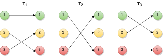
One can then work out composition rules, such as $\tau_i \circ \tau_i = (\tau_i)^2 = e $. Note the exponential notation, and that the rightmost permutation is applied first.
Another interesting group is called the general linear group $GL_n(\mathbb{R})$ of invertible $n \times n$ matrices with real components i.e. with non-zero determinant. If we further require the determinant to be $+1$, we get the special linear group $SL_n(\mathbb{R})$.
As we explore more and more subtleties, we’ll see example of how they relate to groups like these. The advantage of studying underlying structures then slowly becomes clearer.
Subgroups
A subgroup $H$ of a group $G$ is just a subset of $G$ has all the properties of a group, and is closed under $\circ$. In other words, elements don’t hop outside of the subgroup i.e. $a \circ b = c \notin H$, where $a, b \in H$.
In our previous examples, we see that $SL_n(\mathbb{R})$ is clearly a subgroup of $GL_n(\mathbb{R})$: any matrix with determinant $1$ has a non-zero determinant! One can also check it has group properties, for instance the identity matrix.
Cyclic Groups
A cyclic group is one that can be generated from a single element. “Generated” here means applying the group operation on the element with itself. We previously saw that single permutations $\tau_i$ can generate the identity, but they can’t generate other permutations. Hence $S_3$ is not cyclic.
Take the integers $\mathbb{Z}$. This is a cyclic group of infinite order with generator $1$. We write $\mathbb{Z} = \langle 1 \rangle $. It’s worth thinking hard about notation here: with the operation of addition $ \circ = + $, how on earth do we get the negative integers? It turns out the $-$ sign we’re used to is just shorthand. $z^{-1} = -z$ for $z \in \mathbb{Z}$. So in the terminology of “applying the group operation on the element”, we’re actually allowing for negative powers, which is to say applying powers to the inverse $z^{-k} = (z^{-1})^k$. We’ve pretended the generator is alone when in fact we assumed the inverse tags along!
Back to the integers. We say their order is infinite because one can keep adding $1$ and still get a new integer. Let’s look at a cool cyclic group of finite order: the $n^{th}$ roots of unity, where $n$ is the finite order. Recall that a complex number can be represented on the $x, y$ plane, where the $y$ coordinate is the imaginary component. For example $w = 4 + 3i$ is:
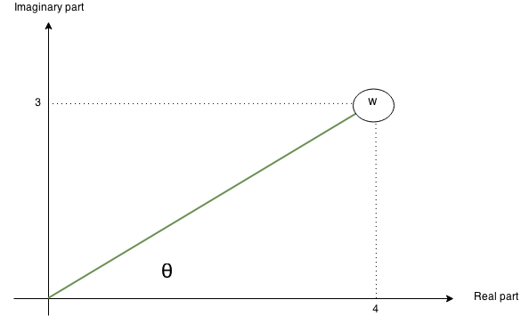
Another, more elegant way of representing $w$ is $r \cdot e^{i \theta}$, where $r$ is the magnitude. In this case $r = 5$, and $\theta = arctan(3/4)$ (good ol’ trig).
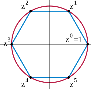
The roots of unity are then the cyclic group generated by $e^{2 \pi i / n}$, where $(e^{2 \pi i / n})^k = e^{2 \pi i (k/n)}$. For $n=6$, we have:
Not only are cyclic groups very pretty, but they also play an essential role in group theory (a role that I am still only beginning to appreciate).
Maps and Morphisms
Cool, so now we have groups. Let’s see what happens when we go from one to another, namely when we consider well-defined maps $m : G \rightarrow G’$. Let’s start with an important propery known as homomorphism. Specifically, a map $m$ is homomorphic if $m(a \circ b) = m(a) * m(b)$. Note that $\circ$ and $*$ are the group operations for $G$ and $G’$ respectively (notation matters!). So what does this property intuitively mean? One way to look at it is such: combining elements in $G$ and then mapping them is the same as first mapping them separately, and then combining them in $G’$. Consider the following example where we transform each element $x \rightarrow x’$ homomorphically in a vector space with vector addition:

Above taking $a + b$ and then mapping the result $c \rightarrow c’$ is equivalent to $ a’ + b’$. This can be useful in settings where we wish to preserve some level of structure accross a transformation, for example in pattern recognition.
An isomorphism is a bijective homomorphism. When two groups are isomorphic, we can essentially hop between one and the other through the isomorphic map. A one-to-one correspondence of elements exists. An automorphism is just an isomorphism of a group to itself i.e. $m: G \rightarrow G$. In other words, it is equivalent to a re-labelling of items.
Conclusion
I meant to talk about kernels, images, centers, and most importantly quotient groups, but this post is getting long. I’ll wait for a post on vector spaces to bring them up, hopefully with some intuitive linear examples! Quotient groups are really where things start getting funky, and are fundamental to modern applications like cryptography.
Hopefully we’ve gotten a sense here of what group theory is about, and glimpsed at some of the potency of such a way of thinking. Check this out next!
Ackowledgements
A huge thanks to anyone contributing to open-source in general, ’tis the best way forward. In this specific case, thanks to Harvard’s online Abstract Algebra course.